Boing! Drawing spherical springs with math
I finally cracked the waveform synthesis of one of the classic laser show abstract effects: the spherical spring, rotating in three dimensions. (Here’s an animated GIF if you’re having trouble viewing the MP4 below.)
Background
Early laser light shows were often played live by the artist driving the laser scanners using a modified analog synthesizer. (They weren’t prerecorded or computer-generated!) It’s an interesting puzzle to reverse-engineer how the effects were created using combinations of simple waveforms.
I took inspiration from Jerobeam Fenderson’s Planets, and his Youtube channel. These are examples of oscilloscope music: music videos where all the visuals are drawn on an oscilloscope directly by the audio waveforms of the music being played. It makes me want to go out and buy a modular synthesizer!
The spherical spring looks so inherently three-dimensional. I thought I needed stuff like rotation matrices or quaternions to generate it. I had only seen the effect in laser shows that were prerecorded, so I didn’t know if there was a simple waveform synthesis behind them, or if they were recorded from a computer. One of Fenderson’s videos seems to show a modular synthesizer programmed to draw the springs, so off we go!
(I couldn’t make out enough of the details of the synth programming in the video to replicate stuff, and I wanted a challenge anyway. It really helped to have the hint that it was possible.)
Details
Edge-on to the equator, it seems easy enough: an amplitude-modulated sine wave inscribed in a circle. (Here, the equator is along the $y$ axis, and the poles are on the $x$ axis.) The square wave cuts off the $y$ axis during the “retrace”, because otherwise the negative half-cycle of the envelope sine wave folds the “fill” wave, causing the trace to double up in a messy way, especially when rotated.
\[\begin{align*} x &= \cos\theta \\ y &= \sin\theta \cdot \sin n\theta \cdot {1\over 2}(1 + \text{square}(\theta)) \end{align*}\]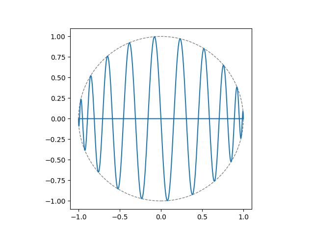
The breakthrough was when I realized that sinusoidal modulation of the $x$ axis is equivalent to $y$-axis rotation: no tricksy rotation matrices or quaternions needed! I went through a few iterations where the effect looked “flat”, until I realized that I was trying to rotate things that were at right angles to each other in the $x$-$z$ plane, so they needed to be modulated in quadrature.
These equations use complex exponentials to be concise and to make the quadrature nature of the waveforms more evident.
\[\begin{align*} z_\text{yrot} &= e^{if_\text{yrot}\theta} \\ z_\text{sph} &= e^{i\theta} \\ z_{\text{fill}} &= e^{in\theta} \cdot \operatorname{Im}\{z_\text{sph}\} \cdot \frac{1}{2} (1+\text{square}(\theta)) \\ x &= \operatorname{Re}\{z_\text{sph}\} \cdot \operatorname{Re}\{z_\text{yrot}\} + \operatorname{Re} \{z_{\text{fill}}\} \cdot \operatorname{Im}\{z_\text{yrot}\} \\ y &= \text{Im}\lbrace z_\text{fill}\rbrace \end{align*}\]I’ve omitted the $z$-axis rotation above, for clarity. That’s a total of three quadrature sine waves (four if you add one for $z$-axis rotation), a square wave synchronized to the sphere envelope, and a small number of multiplications and additions. That does seem within reach of the analog synthesizers back then.
Implementation
I used Matplotlib to animate the effect. I wrote a cheap phosphor decay effect so that a moving object leaves a faint trail, enhancing the sense of motion. Code here on GitHub.
A failed attempt
Here’s an example of where I didn’t realize the $y$-axis rotation needed to be in quadrature. It kind of looks like a distorted flipping coin.